I earlier produced a page
on Chebyshev's inequality in
both its original two-tailed version and a one-tailed version,
another page on the difference
between the mean and mode in a unimodal
distribution, another on Chebyshev
type inequalities for unimodal distributions. This
page considers how the mean, median, mode, and standard deviation
affect each other in a unimodal distribution, and puts a limit on
the median when the mode equals the mean. As ever, comments would
be welcome.
Henry
Bottomley. November 2002.
In September 2006 I added a section and some charts at the end looking at unimodal discrete random variables and how the mean, median, mode, and standard deviation affect each other.
Here is an intriguing part of an abstract taken from S. Basu, A. DasGupta "The Mean, Median, and Mode of Unimodal Distributions: A Characterization", Theory of Probability & Its Applications, Volume 41, Number 2, 1997 pp. 210-223: "For a unimodal distribution on the real line, ... This article explicitly characterizes the three dimensional set of means, medians, and modes of unimodal distributions. It is found that the set is pathwise connected but not convex. Some fundamental inequalities among the mean, the median and mode of unimodal distributions are also derived."
The problem is that the Society for Industrial and Applied Mathematics (SIAM) does not allow access to its electronic publications without subscription. So for amateurs with full time jobs, instead of trailing to a suitable university library to actually read the publication, let us instead consider what this might involve from first principles. If any reader who does have access to the original paper understands the relationship between this note and the results in the original paper, I would be grateful for their comments.
It is widely believed that the median of a unimodal distribution is "usually" between the mean and the mode. However, this is not always true, and (median-mean)/(mode-mean) can in fact take any real value, positive, negative or zero, and (median-mean) can also take any real value even when the mean and mode are equal. We can then use simple linear transformations, changing the location and scale, to produce any point in three dimensional space for (mean, median, mode). Since the resulting set covers the whole space, it is convex, and so cannot be what was intended by the abstract.
So there must be some further restriction on the set beyond its unimodality. Perhaps it is restricted to a given finite range on the real line, restricting the set of points for mean, median and mode to the corresponding cube. A pair of opposite corners of the cube can be reached - just give the random variable a probability of 1 of being at one of the ends of the range. But the other four corners cannot be reached: if the mean is at one end of the range, the mode and median must also be there. The pathwise connected property is easy to show, just by considering the weighted combination of a random variable on the range with a particular mean, median and mode with a uniform random variable on the range to produce a new random variable on the same range: by adjusting the weights continuously, the mean and median can be moved continuously to the mid-range point, while the mode remains unchanged giving a path connection to a line in the cube; and a uniform random variable on the range has its mean and median at the mid-range point while its mode is at any point on the range, giving a path connection along that line.
The lack of convexity is very slightly harder but as an example, if the range is [0,1] then the points (1/4,0,0) and (1/2,1/2,1) for (mean,median,mode) can be reached, or at least approached, while no point on the straight line between them can; for the first consider a distribution with probability 1/2 of being at 0, and probability 1/2 of being distributed uniformly between 0 and 1; for the second, consider a uniform distribution between 0 and 1 with the mode being considered to be at 1 (or an extremely close approximation to this). The proof of this last assertion is not difficult, as only one point need be shown to be impossible and the point a third of the way between them (1/3,1/6,1/3) is not possible: indeed if mean=mode=1/3 then it can be shown that median>=1/4 if the whole continuous unimodal distribution is contained in the range [0,1].
This is interesting, but it seems excessive to restrict the distribution to a finite range. Instead, the rest of this note will assume that the distribution has a finite mean and variance, (and also that it is a continuous random variable with a weakly unimodal distribution, possibly with a point of positive probability at the mode, and possibly with a degree of discretion over selecting the mode), and then consider standardised values which remove the location and scale issues: (median-mean)/standard deviation and (mode-mean)/standard deviation. This reduces the dimensions from three to two, but still produces interesting results.
I have already produced some related results in my other notes. Perhaps the most relevant are the median-mean-mode inequalities in the unimodal case (which can be produced as corollaries of the proof of the one-tailed Chebyshev inequality for unimodal distributions):
|median(X)-E(X)| <= sqrt(3.Var(X)/5)
|mode(X)-E(X)| <= sqrt(3.Var(X))
|mode(X)-median(X)| <= sqrt(3.Var(X))
or rewritten:
-sqrt(3/5) <= (median-mean)/standard deviation <= sqrt(3/5)
-sqrt(3) <= (mode-mean)/standard deviation <= sqrt(3)
-sqrt(3) <= (mode-median)/standard deviation <= sqrt(3)
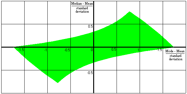
But these inequalities are not sufficient to show the mutual relationship between the three measures of the centre for a continuous unimodal distribution. The following graph of (median-mean)/standard deviation against (mode-mean)/standard deviation shows possible values:

The four "corners" of this shape are not particularly surprising: (sqrt(3),0), (sqrt(3/5),sqrt(3/5)), (-sqrt(3),0), and (-sqrt(3/5),-sqrt(3/5)). Numerically these are (1.73...,0), (0.77...,0.77...), (-1.73...,0), and (-0.77...,-0.77...). The examples given above produce two of these points and reversing the two examples can produce the other two.
Of the four "sides" of the shape, the two shorter sides are convex, and the two longer sides are concave. To demonstrate lack of convexity of the shape as a whole, we only need to find one counter-example. If we draw a straight line joining the ends of the long sides, they will cross the y-axis (i.e. x=0 where the mode is equal to the mean) with y=sqrt(15/16)-sqrt(3/16) or y=sqrt(3/16)-sqrt(15/16), i.e. y=+/- 0.535.... But we can show that when the mode is equal to the mean, the absolute value of (median-mean)/standard deviation must be less than or equal to 1/3 or 0.333.... For the curious still thinking about the cube in the restricted range described above, this maximum absolute value can occur with (mean,median,mode) being (1/4,1/6,1/4) and the standard deviation being 1/4.
We will divide the space into four parts:
Mean<=Median<=Mode
Mean>=Median>=Mode
Mode<Median and Mean<Median
Mode>Median and Mean>Median
Strictly speaking we should also consider the special case of Mean=Median=Mode, but by thinking about a symmetric unimodal distribution of finite variance, it is obvious that by changing the scale, any positive standard deviation can be achieved, thus ensuring that the inequalities are met. (If the distribution collapses to a single point with probability 1 then a standard deviation of zero makes most of the divisions meaningless.)
| Consider a distribution which has a probability
density broadly similar to the red line here. We will produce a new distribution which has the same mean, median and mode, but a smaller variance. First split the red line into three parts: greater than the mode, less than the median, and between the median and the mode. For the part greater than the mode, produce a uniform distribution with the same probability, with the same first moment about the mode, and with the mode as its bottom end (illustrated by the green line greater than the mode): by Lemma 1, this has a second moment about the mode which is no greater. For the part less than the median, produce a uniform distribution with the same probability, with the same first moment about the median, and with the median as its top end (illustrated by the green line less than the median): again by Lemma 1, this has a second moment about the median which is no greater. For the part between the median and the mode, do something similar by produce two uniform distributions with the same total probability, and the same first moment about the mode, with the median as the bottom end with a density equal to the original density at the median and with the mode as its top end (illustrated by the green line between the median and the mode): by a simple variant of Lemma 1, this has a second moment about the mode which is no greater. So the green distribution preserves the total probability (1) and the first moment (mean) of the original while not increasing the second moment or variance. As a next step, make the distribution between the median and mode uniform while retaining the probability; this will reduce (or at least not increase) the first and second moments about the median, and to compensate, squeeze the distribution below the median towards the median so as to restore the original mean of the distribution, again reducing (or not increasing) the second moment about the median, thus producing the purple distribution with the same mean, median and mode and no greater variance. Finally, move the probability greater than the mode into the uniform distribution between the median and the mode, again reducing (or not increasing) the first and second moments about the median, and again squeeze the distribution below the median towards the median so as to restore the original mean of the distribution, reducing (or not increasing) the second moment about the median. This blue distribution has the same mean, median and mode as the original and no greater variance. (Note that the density immediately above the median must be at least as high as the density immediately below the median, since the median is greater than or equal to the mean. In addition, note that if the original mode is equal to the median, the top part becomes a point of positive probability equal to 1/2 at the median.) |
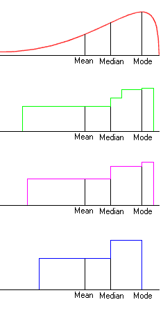 |
The median, mode and mean of this new distribution, together with the property that it is made of two uniformly distributed parts, one of which ranges from the Median up to the Mode and the other down from the Median across the Mean, is sufficient to uniquely determine the distribution and its properties.
Since it has a variance of N2/3 + (N+D)2/3 (where N=median-mean and D=mode-mean) for a given set of mode, median and mean, it provides maxima for the standardised values we are looking at, and part of the boundary of the earlier shape of permitted values.
In particular, for this distribution:
if x=(mode-mean)/standard
deviation
and y=(median-mean)/standard
deviation then:
y=(sqrt(6-x^2) - x)/2
and x2+2xy+2y2=3.
This is an arc of an inclined ellipse centred at the origin, constrained by 0<=y<=x.
The reverse is essentially the same, but with the
distributions reflected and the final lines becoming:
y=( - sqrt(6-x^2) - x )/2and
x2+2xy+2y2=3.
So this is another arc of the same ellipse constrained by x<=y<=0.
We proceed in a roughly similar way to before.
| Again consider a distribution with a density which
looks roughly like the red line here (though the mode may
in fact be lower than the median without affecting the
argument). We will again produce a new distribution which has the same mean, median and mode, but a smaller variance. First split the red line into two parts: less than the mode, and greater than the mode. For each part, produce a uniform distribution with the same probability, with the same first moment about the mode, and with the mode at one end (illustrated by the green distribution): by Lemma 1, these have a second moment about the mode which is no greater than originally. Note that the median of this new distribution is now greater than the original median (if it is not the same), since we have reduced the probability of being between the mode and the original median. Now scale each part of the distribution towards the mode while retaining the original overall mean, producing two uniformly distributed parts so that the median of this further distribution is the original median, preserving the overall mean and mode, and further reducing the variance; this is possible since the mid point between the mode and the top of the range is greater than the median, which in turn is greater than the mean. This final distribution - illustrated in blue - has a minimum variance for a given mean, median and mode and probability for being between the median and mode, but not necessarily the minimum variance for a given mean, median and mode. (Note that if the original mode is almost equal to the median, the top part would again tend towards a point of positive probability equal to 1/2 at the median.) |
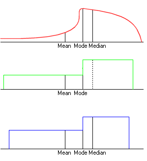 |
Unlike the previous case, this time the median, mode and mean of this new distribution, together with the property that it is made of two uniformly distributed parts joined at the mode, are not sufficient to determine the distribution completely; there are a variety of different distributions with the same properties but different variances and standard deviations. So the aim must be to find the one which minimises the variance and standard deviation. This is not trivial, but doing so produces more of the boundary in the shape above. If N=median-mean, D=mode-mean and Q=probability of being between the mode and the median (note that 0<Q<1/2) then the variance of the blue distribution is:
N2(1+2Q)3/3(1-2Q) + (N(1+2Q)2-D)2/12Q2
This has a derivative with respect to Q of
(8NQ2+2(N-D)Q-(N-D)) (2(N+D)Q+(N-D)) / 6Q3(1-2Q)2
which has two zeros when Q is negative and a more interesting zero at
Q = ( sqrt((9N-D)(N-D)) - (N-D))/8N i.e. when D/N = (1+2Q)(1-4Q)/(1-2Q)
and the derivative is positive for greater Q and negative for smaller Q in (0,1/2), so the minimum variance is
(9N-D)( 9N-D + sqrt((9N-D)(N-D)) )/6 - 9N2 .
In particular, for this minimum variance
distribution:
if x=(mode-mean)/standard
deviation
and y=(median-mean)/standard
deviation then:
y=(27x-x3
+ (x2+9)(3/2))/27(3-x2)
and 3x2-54xy+81y2-27x2y2+2x3y
= 9 .
Unfortunately, this is slightly more complex than a hyperbola,
though it is not difficult to find arcs of hyperbolas which are
close to the arc of the curve constrained by x<y and 0<y.
Note that if mode=mean (i.e. D=0) then the
variance is: N2(1+2Q)3/12Q2(1-2Q)
which is minimised at 9N2 when Q=1/4,
giving a minimum standard deviation of 3N,
implying that when the mode is equal to the mean, Median-Mean <= standard
deviation * 1/3,
and thus proving that the shape is indeed not convex.
The reverse is essentially the same, but with the
distributions reflected and the final lines becoming:
y=(27x-x3
- (x2+9)(3/2))/27(3-x2)
and 3x2-54xy+81y2-27x2y2+2x3y
= 9 .
So this is another arc (on another of the four parts) of the same
complex curve.
| This picture demonstrates the relationship between
the ellipse in red, the four part curve in blue, and in
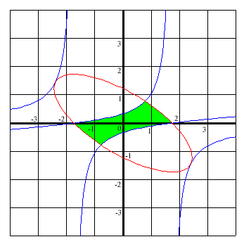
green the possibilities for: x=(mode-mean)/standard deviation and y=(median-mean)/standard deviation . We can put the two results together to say that permitted values must satisfy: x2+2xy+2y2<=3 and 3x2-54xy+81y2-27x2y2+2x3y <= 9. Although the two curves intersect in the four points
we already knew about, they are also mutually tangent at
two more points which we must exclude, namely: |
 |
We have been considering the standardised values
x=(mode-mean)/standard
deviation and
y=(median-mean)/standard
deviation,
and this is illustrated in the green area below.
But we could equally well look at
x=(median-mode)/standard
deviation and
y=(mean-mode)/standard
deviation,
as shown in the purple area, or at
x=(mean-median)/standard
deviation and
y=(mode-median)/standard
deviation,
as shown in the orange area,
thus achieving a slightly different perspective on what are
essentially the same results.

We now have three different inequalities for the absolute difference between the median and the mean:
| In general: | |Median-Mean| <= standard deviation * 1 |
| For a continuous unimodal distribution: | |Median-Mean| <= standard deviation * sqrt(3/5) |
| For a continuous unimodal distribution with the mode and mean equal: |
|Median-Mean| <= standard deviation * 1/3 |
The statements above do not apply to discrete random variables. Consider the following example for a value of d<1/6:
Prob(X=0)=1/2-d
Prob(X=1)=1/2-2d
Prob(X=2)=3d
then Mode(X)=0, Median(X)=1,
E(X)=1/2+4d and Var(X)=1/4+6d-16d2,
and as d tends to 0:
(mode-mean)/standard
deviation tends to -1
while (median-mean)/standard
deviation tends to 1,
which represents a point well outside the shape illustrated
earlier.
So the shape of possible values for discrete unimodal random
variables would be different, but is certainly within the
rectangle above as it is constrained by:
|Median-Mean| <= standard
deviation * 1 and
|Mode-Mean| <= standard
deviation * sqrt(3).
November 2002 .
It is possible to extend this kind of analysis to discrete probability distributions. For example, the Binomial and Poisson distibutions are examples of discrete random variables which have unimodal distributions in the sense that their supports are evenly spaced and the probability mass functions increase up to a particular point (the "mode") and then decrease.
Any value in the chart above that can be achieved for a unimodal continuous distribution can be achieved or at least approached arbitrarily closely with a unimodal discrete distribution since it is possible to produce a sequence of unimodal discrete distributions which converges in distribution to a given unimodal continuous distribution; the reverse is not true as a continuous distribution which approximates closely to a given unimodal discrete distribution will typically not be unimodal itself. So the area identified above should be contained within the equivalent area for discrete unimodal distributions. The chart below illustrates this: the green line shows the boundary for the continuous case and this is within the red area of possible values for the discrete unimodal case.
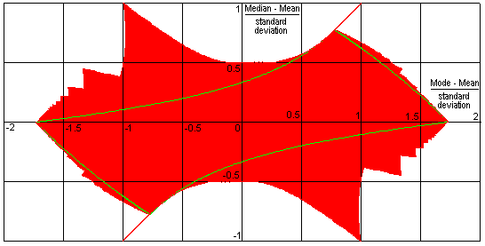
This chart assumes that the mode and median can only take values on the support for the distribution. It would look slightly different if the median could take any values between two points when the cummulative probability up to and including the lower point is exactly ½: the over- and under-hangs would disappear.
In the continuous case, the boundary depended on distributions which were (if you prefer, approached) two uniform distributions joined together. The same is in a sense true for the discrete case, though in some cases an additional point (with a positive but lower probability than its neighbour) is also needed.
As an illustration, consider again the case where the mode is equal to the mean.
The difference between the median and the mean can then be no more than
half a standard deviation in the discrete case
(compared with a third of a standard deviation in the continuous case).
To achieve this, consider five points each with probability 1/20
followed by three points each with probability 1/4, taking the
second last point as the median and the third last point as the mode (it is also the mean).
If these selection of median and mode seems a little arbitrary, then instead consider the
ordered probability distribution:
1/20−3δ,
1/20−2δ,
1/20−δ,
1/20,
1/20+δ,
1/4+4δ,
1/4+δ,
1/4
for small positive δ, and let δ become infinitesimally small.
In 2005 Paul T. von Hippel wrote
Mean, Median, and Skew: Correcting a Textbook Rule in Journal of Statistics Education
Volume 13, Number 2 (2005). He looked at textbooks, many which suggested that
positively skewed distributions would have
mode < median < mean,
i.e. that the median is typically between the mode and the mean.
He noted that "discrete distributions can easily break the rule" and "continuous variables are less likely to break the rule".
The charts above can be interpreted below as confirmation of this, and the charts below try to make this clearer
by dividing the areas between the median, mode and mean as being between the other two.
The substantial increase in the blue (mean between median and mode) and moderate increase in the purple area
(mode between mean and median) which results from moving from the continuous unimodal case to the
discrete unimodal case, compared with the small change in the orange area (median between the mode and mean)
shows that exceptions are easier to find for the discrete unimodal case, but quite possible in either case.
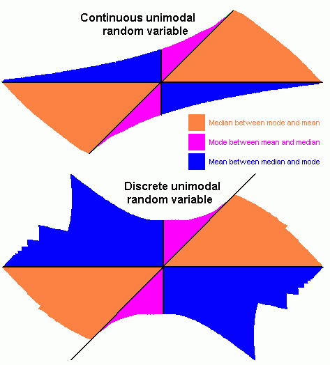
If it seems that the relative areas might have be affected by two quadrants being divided by a diagonal, it is easy enough to use affine transformations such as those used earlier to put the mode or median at the origin; the relative areas would stay the same even when the diagonal became an axis and one of the axes became a new diagonal. The areas should be taken as illustrative, as most distributions encountered in real life will have large standard deviations compared with the differences between the mode, median and mean and so will be represented by points near the origin; symmetric unimodal distributions will be represented by the origin itself; and many discrete distributions will have the mode equal to the median.
Copyright September 2006 Henry Bottomley.
return to top Henry Bottomley's
home page
Chebyshev's inequality Mode-Mean inequality
Statistics Jokes
Chebyshev's
inequalities for unimodal distributions