<= becomes = when distribution X is (for
given k>=1 and any m and any s>0)
P[X=m-k.s] = 1/(2.k2), P[X=m+k.s] = 1/(2.k2),
and P[X=m] = 1-1/k2 .
Note E(X)=m and Var (X)=s2, sd(X)=s, so for this
X P[|X-E(X)|>=k.sd(X)] = 1/k2 .
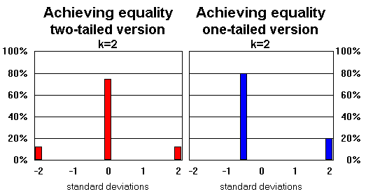
The equality will in general only be achieved for a symmetric
three-valued distribution. If the probabilities are p, 1-2p and p
then equality is achieved when k=(2p)-1/2. A symmetric
two-valued distribution is a special case with k=1.
A chart showing this distribution for k=2 is below.
Note also that for 1>k>0, 1/k2>1 which is not
a probability, so achieving equality would be impossible.
Turning one-tailed version
of Chebyshev's inequality into an equality
<= becomes = when distribution X is (for
given k>0 and any m and any s>0)
P[X=m+s.k] = 1/(1+k2), P[X=m-s/k] = k2/(1+k2) .
Note E(X)=m and Var (X)=s2, sd(X)=s, so for this
X P[X-E(X)>=k.sd(X)] = 1/(1+k2) .
The equality will in general only be achieved for a two-valued
distribution. If the probability of the higher value is p (and
the lower 1-p) then equality is achieved when k=(1/p-1)1/2
A chart showing this distribution for k=2 is below.
Note also that for all k>0, 1>1/(1+k2)>0 so,
unlike the two-tailed version, this is always meaningful.
Markov's inquality states that for Y non-negative and s>0
P[Y>=s] <= E(Y)/s .
If Y=(|X-E(X)|)2 and s=t2 with t>0 then
P[(|X-E(X)|)2>=t2] <= E(|X-E(X)|)2/t2
so P[|X-E(X)|>=t] <= Var(X)/t2
.
If t2=k2.Var(X) for k>0 then k.sd(X)=t
and P[|X-E(X)|>=k.sd(X)] <= 1/k2 .
Proof of one-tailed
version of Chebyshev's inequality
If P[X-E(X)>=t] = 0 for given t>0 then clearly
true,
otherwise let a = P[X-E(X)>=t], noting 0<a<1,
and b = E(X-E(X)|X-E(X)>=t), noting t<=b,
and c = E((X-E(X))2|X-E(X)>=t), noting t2<=c<Var(X)/a
Consider T=t if X-E(X)>=t and T=0 if X-E(X)<t and
consider S=0 if X-E(X)>=t and S=(X-E(X)).t/b if X-E(X)<t :
then E(T) = a.t and E(S) = -a.b.t/b = -a.t
and E(S|X-E(X)<t) = -a.t/(1-a)
and
E(T2) = a.t2 <= a.c
and E(S2) = (Var(X)-a.c).t2/b2 <= Var(X)-a.c ,
so Var(X) >= E(T2)+E(S2) ;
but E(S2) = (1-a).E(S2|X-E(X)<t) >= (1-a).(E(S|X-E(X)<t))2=a2.t2/(1-a)
so Var(X ) >= a.t2+a2.t2/(1-a) = a.t2/(1-a) ,
so a <= 1/(1+t2/Var(X))
so P[X-E(X)>=t] <= 1/(1+t2/Var(X))
i.e. P[X-E(X)>=t] <= Var(X)/(Var(X)+t2) . If t2=k2.Var(X) for k>0 then k.sd(X)=t
and P[X-E(X)>=k.sd(X)] <= 1/(1+k2) .
Alternative proofs of one-tailed version
The proof above was mine. A.G.McDowell has two at his page on Chebyshev's
Inequalities: one of his own and one from 'Probability
and Random Processes', by Grimmett and Stirzaker, published
by Oxford Science Publications, ISBN 0 19 853665 8. The latter
has the advantage of being short and (slightly adapted) is
something like this:
With t>0, for any c>=0 P[X-E(X)>=t] = P[X-E(X)+c>=t+c]
<= E((X-E(X)+c)2/(t+c)2) = (Var(X)+c2)/(t+c)2.
But treating (Var(X)+c2)/(t+c)2 as a
function of c, the minimum occurs at c = Var(X)/t,
so P[X-E(X)>=t] <= (Var(X)+Var(X)2/t2)/(t+Var(x)/t)2
= Var(X)/(t2 + Var(x)).
Pafnuty Lvovich Chebyshev was a notable Russian mathematician,
who was born on 16 May 1821 and died on 8 December 1894. He wrote
on number theory, analysis, probability, mechanics and maps.
Being Russian, his name was written in the Cyrillic alphabet,
causing problems of translitteration. Stijn van
Dongen has compiled a list of 33 western European verions of
his surname, of which Chebyshev seems to be the most popular in
English, Tchebycheff in French, Cebysev in Spanish, and
Tchebyscheff in German. Despited this variety, the final vowel
always seems to be transcribed as "e" in that list when
it is in fact pronounced "yo" in Russian. Even his
given name and his patronimic have varying versions in roman
script.
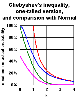
The two inequalities are very similar in form. However, for
small k, they produce very different results. Indeed the one-tailed
version produces meaningful results for 0<k<1, while
Chebyshev's inequality less helpfully limits the probability to
being less than or equal to a number greater than 1. For k=1, the
one-tailed version provides the result that the median of a
distribution is within one standard deviation of the mean. For
large k, as shown in the table and chart below, the mamimum
probability values given by the two inequalities are very similar.
For large k, they are very different to the results for the
Normal distribution.
P(|X-E(X)|>=k.sd(X))
or P(X-E(X)>=k.sd(X))
k
Chebyshev's
inequality
One tailed
version
Normal
two-tailed
Normal
one-tailed
0.1
(10000%)
99%
92.0%
46.0%
0.5
(400%)
80%
61.7%
30.9%
0.9
(123%)
55%
36.8%
18.4%
1
100%
50%
31.7%
15.9%
1.64
37.0%
27.0%
10%
5%
1.96
26.0%
20.7%
5%
2.5%
2
25%
20%
4.55%
2.28%
3
11.11%
10%
0.27%
0.13%
4
6.25%
5.88%
0.006%
0.003%
4.36
5.26%
5%
0.0013%
0.0007%
4.47
5%
4.76%
0.0008%
0.0004%
9.95
1.01%
1%
close to 0
close to 0
10
1%
0.99%
close to 0
close to 0
The similarity of the probability values for high k between
Chebyshev's inequality and the one-tailed version is slightly
misleading, as can be seen when the distribributions which turn
the inequalities into equalities are considered, with examples in
the chart below. The equality distribution for Chebychev's
inequality is symmetric, while the equality distribution for the
one-tailed version is not. For large k, the highest element of
the former has only just over half the probability of the highest
element of the latter.
"This goes back more than a century. I do not know
the history.
"This is the simplest of a class of inequalities,
which I believe are due to Markov, a student of Chebyshev. A good
book on the moment problem should have a reference.
If 1=m_0, m_1, ..., m_{2n} are the first 2n moments of a
probability distribution,
let f be the unique (apart from a constant of proportionality)
polynomial of degree at most n+1 with x as a root, and orthogonal
to all polynomials of degree less than n.
If x is not a root of the orthogonal polynomial of degree n,
there are n+1 roots, and the unique distribution concentrated at
these roots fitting the given moments maximizes P(X <= x) and
minimizes P(X < x).
If x is a root of the orthogonal polynomial, the 2n-th moment may
not be matched at the n roots.
"In the case n=1, If x=E(X), the extreme distribution
is concentrated at E(X).
Otherwise, if x = E(X)+t, the distribution is concentrated at x
and E(X)-Var(X)/t."
Copyright June 1999 Henry Bottomley. All
rights reserved.
Some extra
thoughts on Chebyshev type inequalities for unimodal
distributions (October 1999):
If X is a continuous random variable with a
unimodal probability density function (pdf), we may be able to
tighten Chebyshev's inequality, though only by adding some
complexity.
If the unimodal probability density function is
also symmetric, then result P[|X-E(X)|>=t] <= 4.Var(X)/(9.t2)
or P[|X-E(X)|>=k.sd(X)] <= 4/(9.k2)
applies for all t,k>0 This is Gauss's inquality of 1821 when the mode and mean are
identical,
and is four ninths of the bound of Chebshev's inequality.
When 0<t2<=4.Var(X)/3
or 0<k<=2/sqrt(3) about 1.15470...
I think this can be improved to
P[|X-E(X)|>=t] <= 1-t/sqrt(3.Var(X)) or P[|X-E(X)|>=k.sd(X)] <= 1-k/sqrt(3) It is obvious that for a symmetric pdf, the one-sided bounds
are half these.
If the unimodal pdf need not be symmetric then I
suspect the inequality only applies for high t and k:
whent2>=B2.Var(X)
or k>=B where B is the largest root of 7.x6-14.x4-x2+4=0,
about 1.38539...
P[|X-E(X)|>=t] <= 4.Var(X)/(9.t2)
or P[|X-E(X)|>=k.sd(X)] <= 4/(9.k2)
as before,
butwhen 0<t2<=B2.Var(X)
or 0<k<=B and with B as before,
about 1.38539...
P[|X-E(X)|>=t] <= 1-(4.t2/(3.(Var(X)+t2)))2or P[|X-E(X)|>=k.sd(X)] <= 1-(4.k2/(3.(1+k2)))2 (I produced a sketch
of why this is true in 2002)
The one sided version might be:
when t2>=5.Var(X)/3
or k>=sqrt(5/3), about 1.29099... P[X-E(X)>=t] <= 4.Var(X)/(9.(Var(X)+t2))
or P[X-E(X)>=k.sd(X)] <= 4/(9.(1+k2)) this time four ninths of the one sided version of Chebyshev's
inequality
and when 0<t2<=5.Var(X)/3
or 0<k<=sqrt(5/3)
P[X-E(X)>=t] <= 1-4.t2/(3.(Var(X)+t2))
or P[X-E(X)>=k.sd(X)] <= 1-4.k2/(3.(1+k2))
(I have attempted a proof
of this in 2001)
In an e-mail in October 2000, Michael Dummer commented: "there is a simple unimodal distribution which meets the
tighter Unimodal Chebyshev bound: a rectangular or uniform
distribution with an impulse at the midpoint of the uniform range."
I responded:
"I think this applies to the symmetric unimodal case; for
the non-symmetric unimodal two and one-sided cases, the bound is
met for uniform distributions with an impulse away from the
midpoint." Perhaps I should have added the bounds for small t
and k are achieved for a uniform distribution
with an impulse at one end where the probability of the uniform
distribution is 4.k2/(3.(1+k2)).
I have developed a page
which takes the one-tailed case a little further (especially the
unimodal case) as well as some median-mean-mode inequalities.